research
Here are some summaries of my research work.
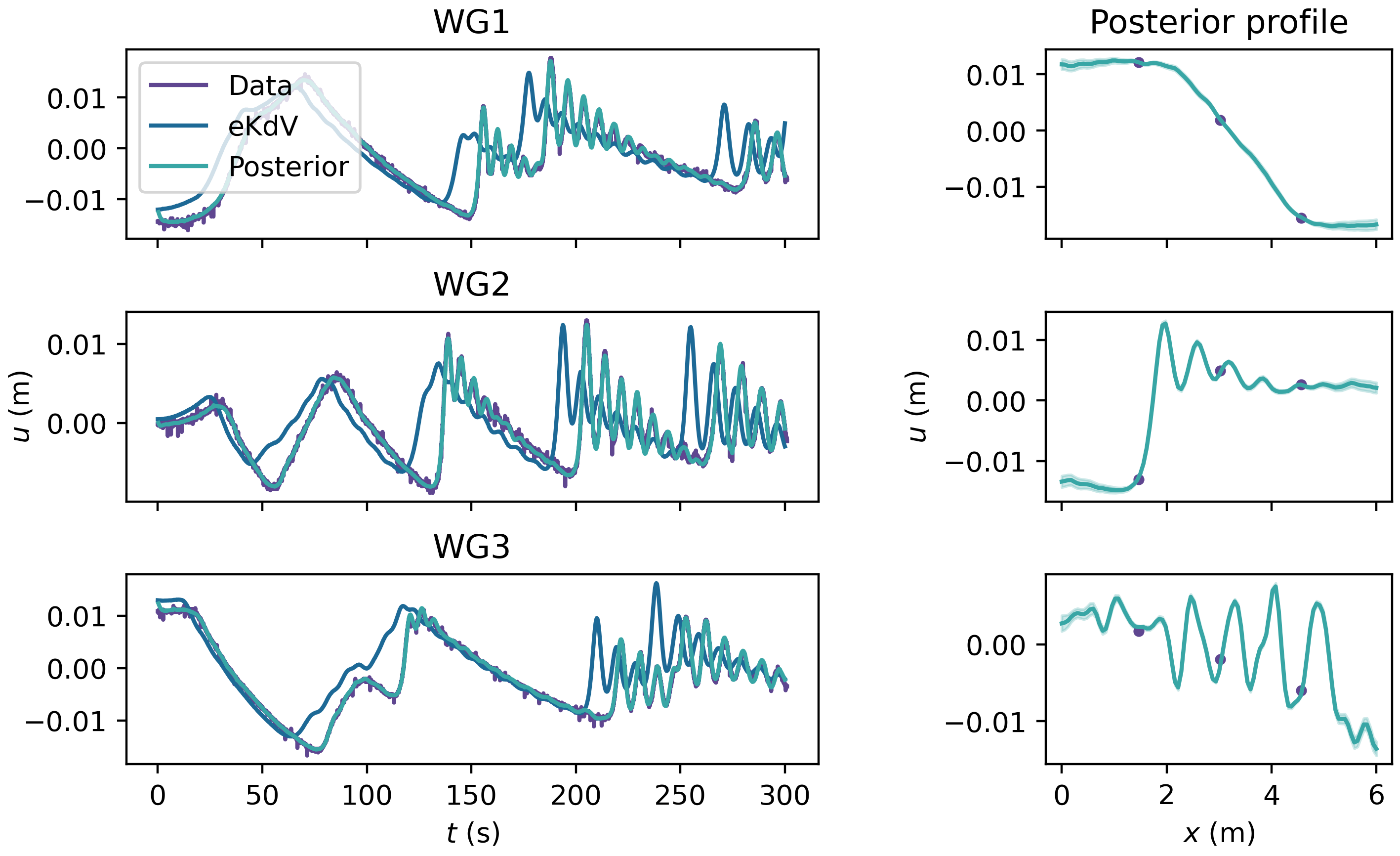
statFEM for nonlinear problems
The statFEM is a methodology to synthesise finite element models with data. Our work extended this to nonlinear, time-dependent PDEs, with low-rank covariances for scalable computation (see here and here). We take a nonlinear, time-dependent PDE:
\[ u_t + \mathcal{L} u + \mathcal{F}(u) = \xi, \]
\(u := u(x, t)\), \(x \in \mathcal{D} \subseteq \mathbb{R}^d\), \(t \in [0, T]\), and embed a Gaussian process \(\xi \sim \mathcal{GP}(0, \delta(t - t') \cdot k(x, x'))\) inside of PDE, to capture structural model imperfection.
If we discretise the above then we can write out a transition density \(p(u_h^n | u_h^{n - 1}) = \mathcal{N}(\mathcal{M}(u_h^{n - 1}), G)\), where \(u_h^n\) is our finite element discretised solution, at time \(n\Delta t\). Combining with an observation model allows for general nonlinear filtering. If we have a linear Gaussian observation model then we get something like:
\[ \begin{aligned} p(u_h^n | u_h^{n - 1}) &= \mathcal{N}(\mathcal{M}(u_h^{n - 1}), G), \\ p(y_n | u_h^{n - 1}) &= \mathcal{N}(H(u_h^n), \sigma_n^2 I). \end{aligned} \]
This permits the usual nonlinear filtering (like the ensemble Kalman filter or the extended Kalman filter), which computes the posterior \(p(u_h^n | y_{1:n})\).